MUMT 307 — Max Henry

Background: Modal Synthesis

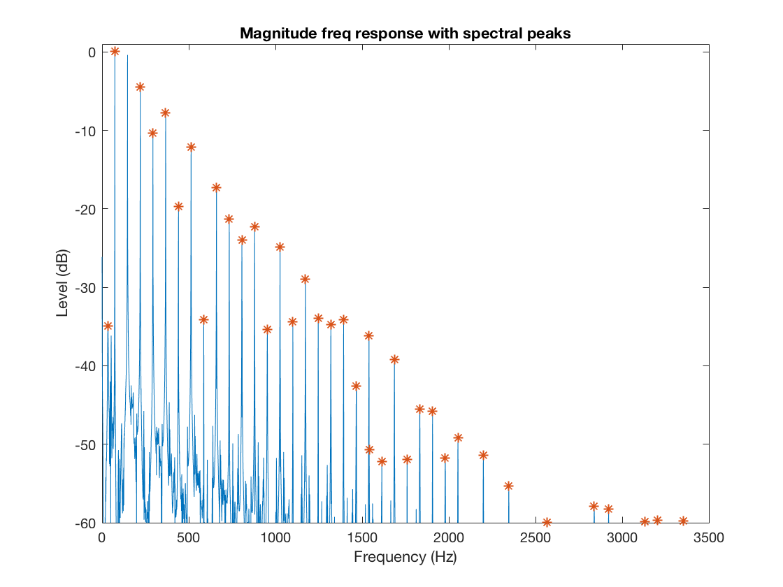
Modal synthesis offers a relatively simple method of reproducing pitched percussive sounds. By measuring the peaks and corresponding bandwidths of a given sound spectrum, a bank of resonant filters can be designed such that when excited by an impulse or “residual signal” they reproduce (roughly speaking) the original signal. Using resonant filters allows for an approximation of both the spectral and temporal profile of a decaying sound: the radius of a given filter, correlating to its bandwidth, also determines its decay time. In this way each partial of the resultant sound has its own decay time corresponding to its relative gain.

The idea of this project was simple: design an engine that can analyze a single note wave file (for example, of a Rhodes keyboard) for its resonant modes, build a filter-bank to emulate that sound, and then scale and shift resultant filters to reproduce the same timbre at a variety of pitches and velocities. In other words: generate a full instrument with the character of a given sample from a single recorded note.

Matlab -> STK

I decided to write as much as the project as possible in STK because it would be a challenge. Before this semester I had no coding experience in C++, and I knew that writing the project in STK would force me to get more familiar with the language. As a result almost every step of the way proved to be a much greater challenge than I had anticipated. It was decided fairly early on that the modal analysis would take place in MATLAB. It was then a matter of figuring out how to get that information to my C++ engine.

The MATLAB script finds modal resonances using the findpeaks function on the FFT of the source signal. The frequency values and magnitudes are then refined using parabolic interpolation. Starting from each local maxima, a for loop “crawls down” until a drop in 3dB has been located — from here I take an approximation the 3dB bandwidth, and calculate the corresponding radius value.

The resultant filter-bank information — in triplets of frequency, radius, and gain — is stored in a CSV file FreqsRs.csv to be passed to the synthesis engine.

Getting into C++

Passing information to a C++ program proved to be much more difficult than I anticipated. It took some trial and error before I settled on using a CVS file as output from MATLAB. In this way I could call the getline() function in two loops: one to cut the input by rows (each row containing an array of parameter values — e.g. all the frequencies), and one to sort it by comma separated values.

I needed to ensure that the code could accommodate a filter bank of any size. Thanks are due to Harish Venkatesan for introducing me to vectors — push_back facilitated this necessity. Thanks are also due to fellow special-undergrad Graham Smith for introducing me to classes. The following code excerpt reads frequency, radius and gain values from the file stream and pushes them back into a vector of the “filtParam” class.

The idea Behind the Engine

The inspiration for this engine came from playing around with a newly completed script for Homework 8, of which this script is a modification. We were asked to reproduce a sound by modal analysis and synthesis. I found by scaling the frequencies of the modes I could easy transpose the resynthesized note, which scaled within about +/- 12 semitones with a pretty reasonable fidelity to the original signal.

The most exciting discovery was realizing that by selectively turning off the upper resonant filters while gaining down the signal output, I could emulate a fairly musical velocity note response. Using this mechanic, quieter notes have less overtones. This is an idea I would go on to develop in the C++ implementation, by using a scaling curve to selectively gain down the upper partials rather than cutting them off completely. Curve design would end up taking up quite a lot of my time on this project; I’ve implemented curves having to do with gain, pitch and envelope scaling — surprisingly tuning these curves turned out to be an incredibly musically rewarding activity, playing into my experience as a sound designer.

Curve Design

An unexpected benefit of working with MATLAB was being able to prototype and visualize velocity and pitch related scaling curves.

It was decided fairly early on to have a differential “overtone curve” that takes both note velocity and a stretch factor into account. “Stretch factor,” represented in the C++ code as stretch and in the equation below as sigma represents the distance between the desired output pitch and the specified pitch of the input sample note.

Overtone gain (letter g at partial p out of a total P partials, with velocity v) is calculated as above. The sigma value, above right, effectively damps the velocity for higher note values. It’s worth noting that the effect is unidirectional, i.e. it doesn’t amplify notes below the specified sample note-in value.

This particular equation was arrived at by an iterative three step process: (1) first by sketching the desired curve by hand, then (2) using MATLAB to approximate the curve based on desired input variables (number of filters, velocity, note in and note out), and finally (3) by implementing the code in C++ and listening to the results. As I mentioned above this was a very musically rewarding process.

Some examples of the curve can be seen below, using a test P value of 38.

Here are some other curves I played with, mostly concerned with scaling via pitch.

The Envelope

I decided on a three stage attack-decay-release exponential amplitude envelope (implemented here with stk’s asymp). Even though resonant filters will decay on their own (they produce damped sinusoids when “impulsed”) I wanted a way to (1) truncate notes in a relatively natural way on note-off events (here simulated by the note duration value) and (2) attenuate the sustain of higher (i.e. more “stretched”) notes.

The amp decay was implemented simply, with reference to the earlier “stretch” value (notein/noteout). An attack time of 0.1s was chosen to mask the initial “click” of the impulse exciting the filter-bank. The release value of 0.4 was set simply to be the most musical “damping,” and was roughly based on empirical measurements of piano release lengths.

Error Checking

My code implements very simple error checking. It makes sure that the values are within certain reasonable bounds. Thanks are due again to Harish for introducing me to in line conditionals.

DEMOS — Rhodes, Piano, XYlophone, Marimba at three velocities

Results

We have a robust engine that can reproduce pitched percussive sounds fairly well. The Rhodes and marimba emulations are particularly strong. The piano, while far from realistic, has a charming character to it reminiscent of the YAMAHA CP80 on early jazz fusion records. The xylophone has a peculiar metallic character, but is included to demonstrate the breadth of samples that are easily emulated. As is typical of modal synthesis, sustained instruments (such as violins, organs) are not modelled well by this engine.

Next Steps

There are a few things I’d like to get sorted moving forward.

(1) There’s an issue with the gain — because the program is synthesizing from a potentially infinite variety of filter banks, there has to be some programmatic implementation of internal limiting. This may have to happen on the MATLAB/analysis side of things. For now I am normalizing by the total number of filters, and the output is rather quiet as a precautionary measure.

(2) Midi implementation — of course that’s the whole point of this instrument! I’m positive the musical velocity scaling will come alive with a nice midi controller. I’d love to hear how the rhodes/pianos sound as real, playable instruments.

(3) I never really managed to get the pitch stretching to scale in a way that feels natural over about one octave in either direction. This may be too much to ask of information from a single note sample — that said I’m positive there are more musical curves out there, and with a little experimentation we can stretch these filter-banks a lot further without sounding unnatural.

THANK YOU FOR YOUR INTEREST.

Instructions

<<What follows is an adapted version of the README available on the github project page.>>

Note:: the synthesis toolkit (stk) is required to compile the C++ code. https://ccrma.stanford.edu/software/stk/

(-1) Download and expand modalengine.zip — it shouldn’t matter where this is on your computer, so long as all of the contents stay within this subdirectory.

(0) If you haven't already, compile the C++ code. You will need STK, and you will need to specify both the include and library paths. Here's how this looks on my machine (you will have to change the paths as necessary):

g++ -I/Users/maxsolomonhenry/Documents/cprojects/stk-4.6.0/include/ -L/Users/maxsolomonhenry/Documents/cprojects/stk-4.6.0/src/ -D__MACOSX_CORE__ 307finalWAV.cpp -lstk -lpthread -framework CoreAudio -framework CoreMIDI -framework CoreFoundation

(1) Run the MATLAB code, taking care to specify which .wav file you want analyzed in the audioread function (line 18). Example sounds can be found in the "examples" directory. This will output a csv file to be read by the C++ component.

(2) Run the compiled code with the following specifications:

./a.out <notein> <noteout> <velocity> <duration>

Where <notein> is a value from 0-127 indicating the midi pitch of the analyzed sample,
<noteout> is a value from 0-127 specifying the desired output pitch (also in midi),
<velocity> is a value from 0-127 indicating note output velocity (higher = louder and more overtones), and
<duration> is a value from 0.1 - 6 indicating the desired note duration time in seconds.

***note, please don't use the < > brackets when passing your parameters!

(3) Enjoy.

Modal analysis and resynthesis engine for matlab/stk